Abstract
A one-paragraph abstract summarizing the article. Replace this placeholder with a concise description of the problem, approach, and key findings.
Introduction
Welcome to this article. This section introduces the topic and explains who the article is for and how it is organized.
Who This Article Is For
This article is for anyone interested in the topic.
How to Read This Article
Each section builds on the previous one. Start from the beginning and work through to the end.
Getting Started
This section introduces the fundamental concepts.
Overview
Provide an overview of the topic here.
Key Concepts
Explain the key concepts that readers need to understand. This article builds on tools from the scientific Python ecosystem, including NumPy Harris et al., 2020, SciPy Virtanen et al., 2020, and Matplotlib Hunter, 2007. For a broader introduction to data analysis in Python, see McKinney (2022), which builds on ideas introduced by McKinney (2010) for reproducible scientific computing.
print("Hello, World!")Key Tools
The table below shows an overview of the key tools used in this article.
Table 1:Overview of key tools.
Tool | Description | Version |
|---|---|---|
Python | Programming language | 3.12 |
NumPy | Numerical computing library | 1.26 |
Matplotlib | Plotting and visualization | 3.8 |
MyST | Markdown authoring framework | 1.8 |
Installation
This section covers how to set up your environment.
Prerequisites
List the prerequisites here.
Installation Steps
pip install numpy matplotlibVerifying the Installation
import sys
print(f"Python version: {sys.version}")
Example
This section walks through a complete example.
Setting Up
Describe the setup steps here.
Sample Figure
Figure 1 shows a sample bar chart generated with Matplotlib.
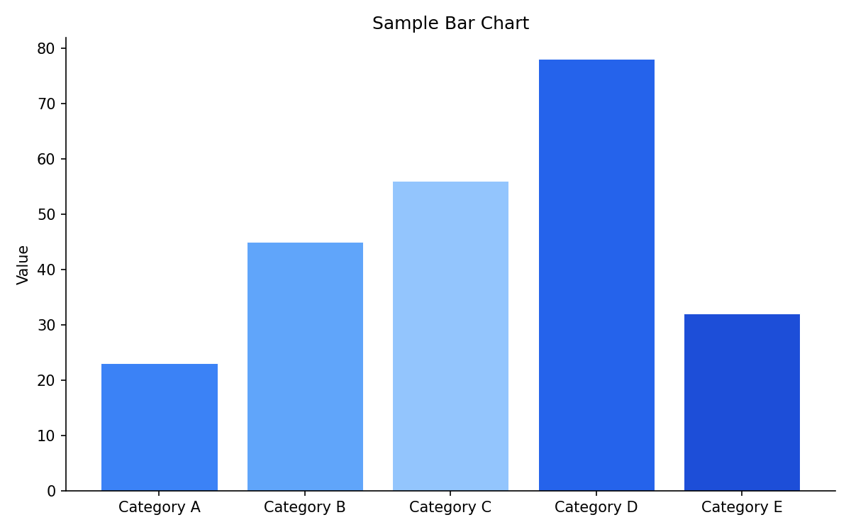
Figure 1:A sample bar chart showing values for five categories.
Running the Example
import numpy as np
import matplotlib.pyplot as plt

x = np.linspace(0, 2 * np.pi, 100)
y = np.sin(x)

fig, ax = plt.subplots()
ax.plot(x, y)
ax.set_xlabel("x")
ax.set_ylabel("sin(x)")
ax.set_title("A Simple Plot")
plt.show()
Conclusion
This article demonstrated the basic workflow. Replace this section with your own conclusions and next steps.
Acknowledgments
Thank you to everyone who contributed to this article.
- Harris, C. R., Millman, K. J., van der Walt, S. J., Gommers, R., Virtanen, P., Cournapeau, D., Wieser, E., Taylor, J., Berg, S., Smith, N. J., Kern, R., Picus, M., Hoyer, S., van Kerkwijk, M. H., Brett, M., Haldane, A., del Río, J. F., Wiebe, M., Peterson, P., … Oliphant, T. E. (2020). Array programming with NumPy. Nature, 585(7825), 357–362. 10.1038/s41586-020-2649-2
- Virtanen, P., Gommers, R., Oliphant, T. E., Haberland, M., Reddy, T., Cournapeau, D., Burovski, E., Peterson, P., Weckesser, W., Bright, J., van der Walt, S. J., Wilson, J., Millman, K. J., Mayorov, N., Nelson, A. R. J., Jones, E., Kern, R., Larson, E., Carey, C. J., … van Mulbregt, P. (2020). SciPy 1.0: Fundamental algorithms for scientific computing in Python. Nature Methods, 17, 261–272. 10.1038/s41592-019-0686-2
- Hunter, J. D. (2007). Matplotlib: A 2D graphics environment. Computing in Science & Engineering, 9(3), 90–95. 10.1109/MCSE.2007.55
- McKinney, W. (2022). Python for Data Analysis (3rd ed.). O’Reilly Media.
- McKinney, W. (2010). Data structures for statistical computing in Python. Proceedings of the 9th Python in Science Conference, 56–61. 10.25080/Majora-92bf1922-00a